Let’s try to understand Bayesian optimization from the basic perspective of the Bayesian approach.

Basic Concept

What is the Bayesian Approach?

• The parameter $\theta$ is considered a “realization of some random variable $\theta$.” After assuming a probability distribution for $\theta$ (prior distribution), the distribution of $\theta$ is updated through information obtained from random sampling (posterior distribution).
• Typically, “prior information” about $\theta$ is used, and the method gradually improves the prediction of $\theta$ by incorporating posterior data obtained through sampling.

Hyperparameter Tuning

Concept

Hyperparameters are external configuration variables used by data scientists to manage machine learning model training. Sometimes referred to as model hyperparameters, they are manually set before model training. Unlike parameters, which are derived automatically during the training process, hyperparameters are set by the data scientist.

Examples of hyperparameters include the number of nodes and layers in a neural network or the number of branches in a decision tree. Hyperparameters determine key features of a model such as architecture, learning rate, and model complexity.

Types of Hyperparameter Tuning

What are the techniques for hyperparameter tuning?

There are numerous hyperparameter tuning algorithms, but the most commonly used ones are Bayesian optimization, grid search, and random search.

Bayesian Optimization
Bayesian optimization is based on Bayes’ theorem, which explains the likelihood of an event occurring related to existing knowledge. When applied to hyperparameter optimization, the algorithm builds a probabilistic model of hyperparameter sets that optimize a specific metric. It uses regression analysis to iteratively select the best hyperparameter set.

Grid Search
In grid search, the algorithm works through all possible combinations of a specified list of hyperparameters and performance metrics to determine the best one. While grid search works well, it can be tedious and computationally intensive, especially when dealing with a large number of hyperparameters.

Random Search
Random search is based on similar principles as grid search, but instead of evaluating all combinations, it randomly selects groups of hyperparameters in each iteration. It works well when a relatively small number of hyperparameters primarily determine the model’s outcome.

In this column, we will focus on Bayesian optimization.

Application

Let’s assume that the objective function we need to optimize is $f(x|\theta)$.
In real-world scenarios, the variable $\theta$ is likely to be multivariate.
Let’s call the prior distribution of $\theta$, $\xi(\theta)$.

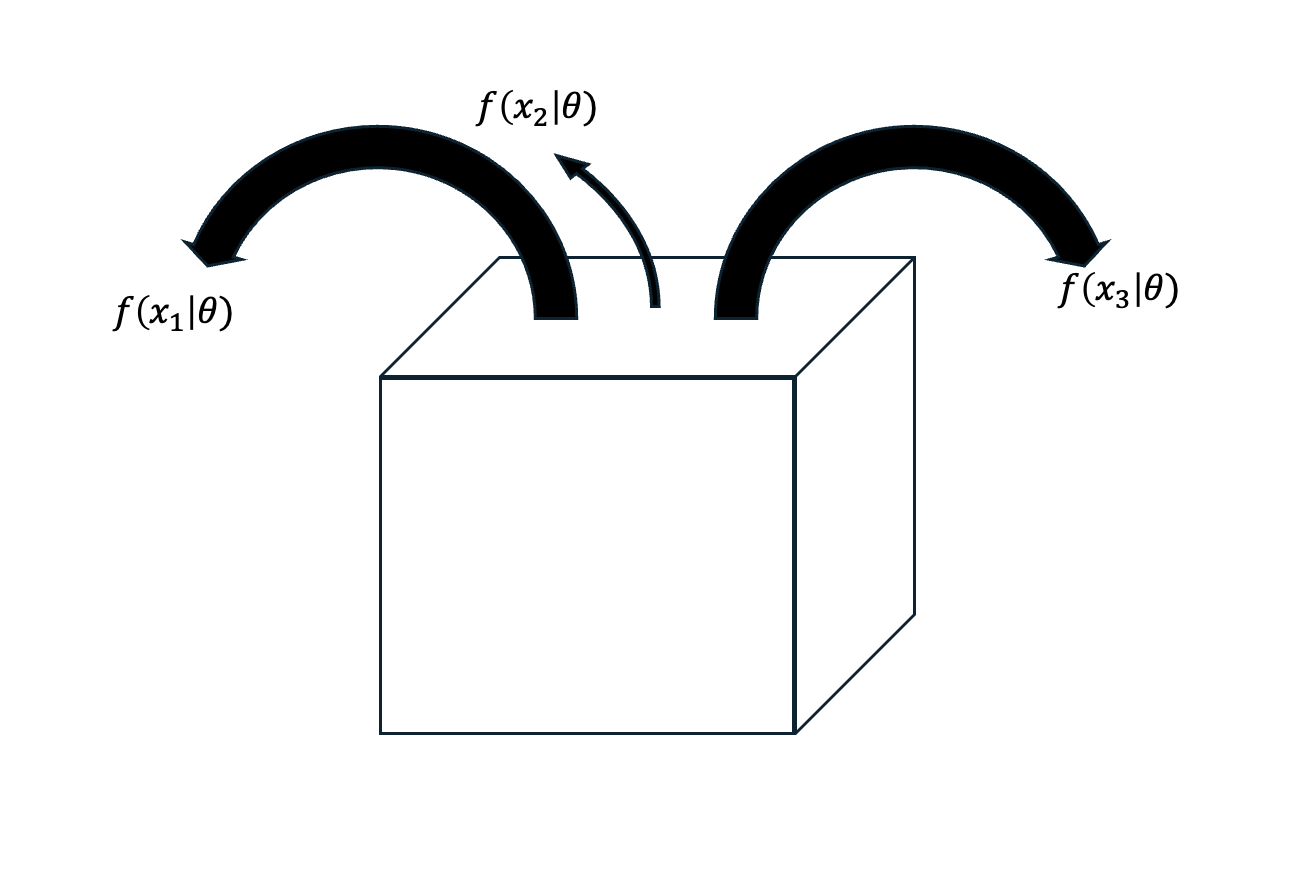
Now, imagine we sample ${x_1, x_2, … x_n }$ from a population as shown in the diagram below:

Then the posterior distribution becomes $\xi(\theta|x_1, x_2, … x_n)$.
This is the basic idea behind the Bayesian approach. To obtain the posterior distribution following the Bayesian method, we use the formula:

This process shows that we must know both $\xi({\theta})$ and $f_n$.

However, one challenge in optimization is that we often deal with a black-box function, where the distribution of $f$ is unknown.

At this point, we can use a Gaussian Process to make an estimation. We’ll cover the detailed theory behind Gaussian Processes later.

https://stats.stackexchange.com/questions/532073/bayesian-optimization-vs-gradient-descent

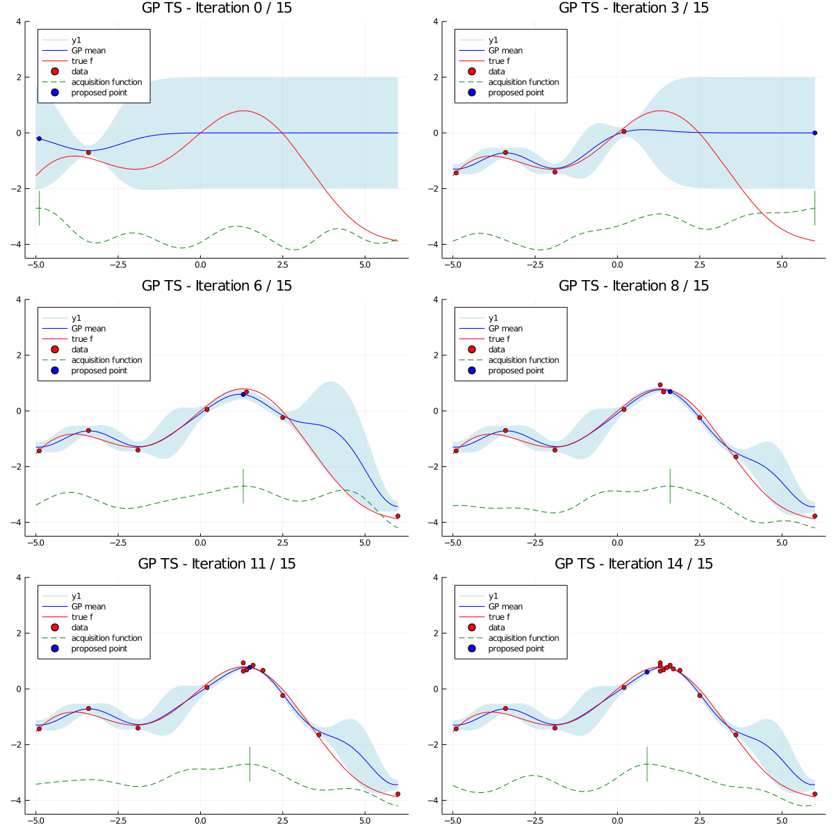
In Bayesian optimization, we set up a surrogate model and an acquisition function.
The surrogate model estimates the approximate value of $f(x|\theta)$ based on the inferred results thus far. The acquisition function identifies the point most likely to yield a higher value than those observed so far, based on the probabilistic distribution inferred by the surrogate model. The above diagram provides an intuitive visual of this process.

So, how do we find the point where the acquisition function reaches its maximum?
We achieve this through Exploration and Exploitation:

• Exploration: Seeking areas of high uncertainty, assuming that a higher value might be found there.
• Exploitation: Focusing on areas near previously observed high values, assuming that a higher value might be found close by.

Through this approach, we can understand Bayesian optimization via the Bayesian method. Although we didn’t dive deeply into Gaussian Processes, I hope this discussion provides insights into the approach and mindset needed when dealing with posterior distribution of unknown functions in real-world applications.