FLEXTRON: Many-in-One Flexible LargeLanguage Model
Published in , 2024
Today, I will summarize the paper titled “FLEXTRON: Many-in-One Flexible Large Language Model.” The primary focus of this paper is to propose a novel framework with an elastic structure that can quickly adapt to diverse user environments. To achieve this, paper suggests that like Mixture-of-Experts.
Background and Notation
Elastic Multi-Layer Perceptron(MLP)
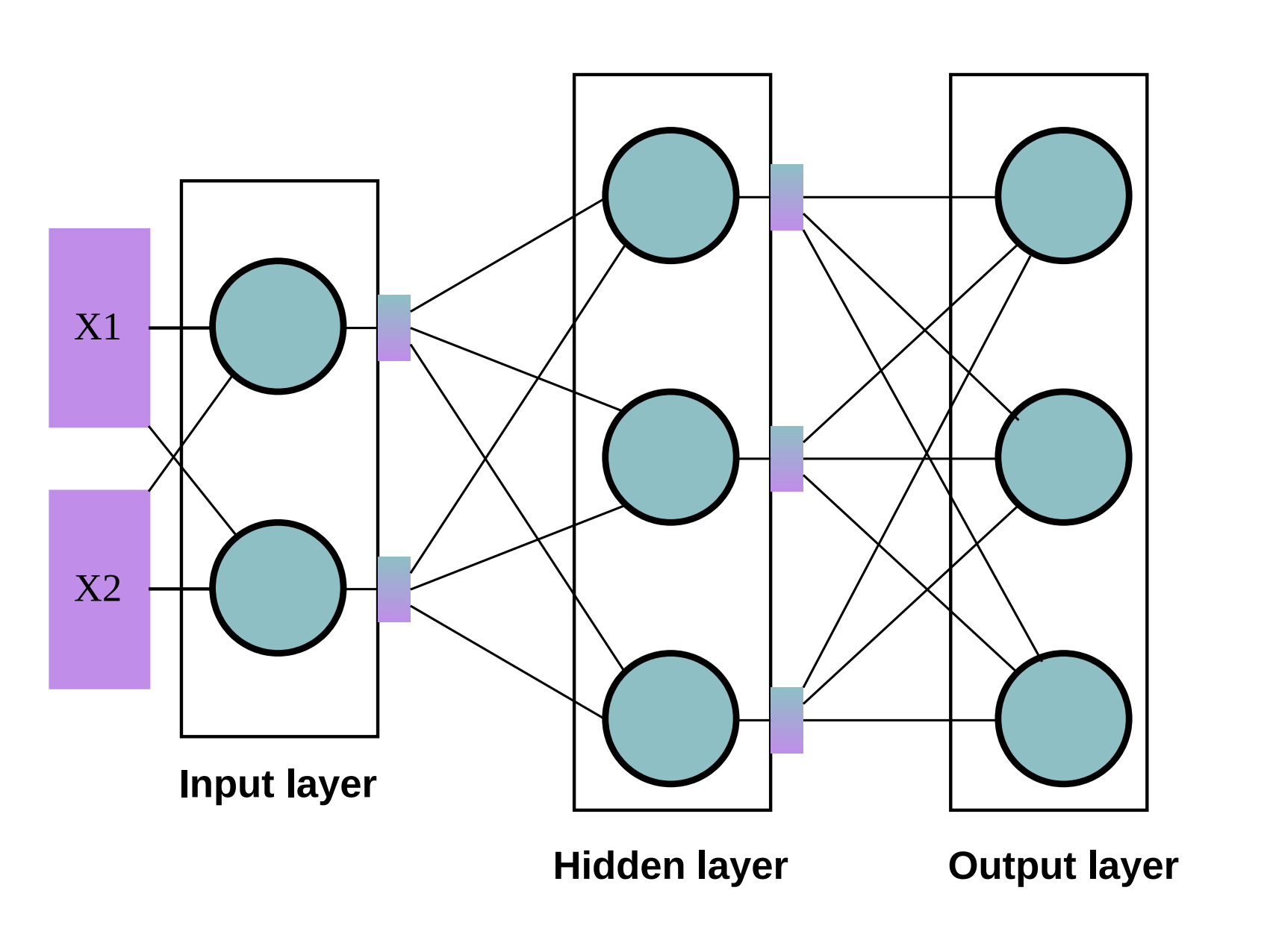
 Suppose we have a Multi-Layer Perceptron (MLP) with a single hidden layer. In a typical MLP, all neurons in the hidden layer are always activated during computation. - Input: $X_1$, $X_2$
- Each input is passed to every neuron in the hidden layer through the weight matrix $W^{(1)}$. - The activation function (e.g., Sigmoid, ReLU) is applied to the hidden layer outputs. - The results are then passed to the output layer via the weight matrix $W^{(2)}$.
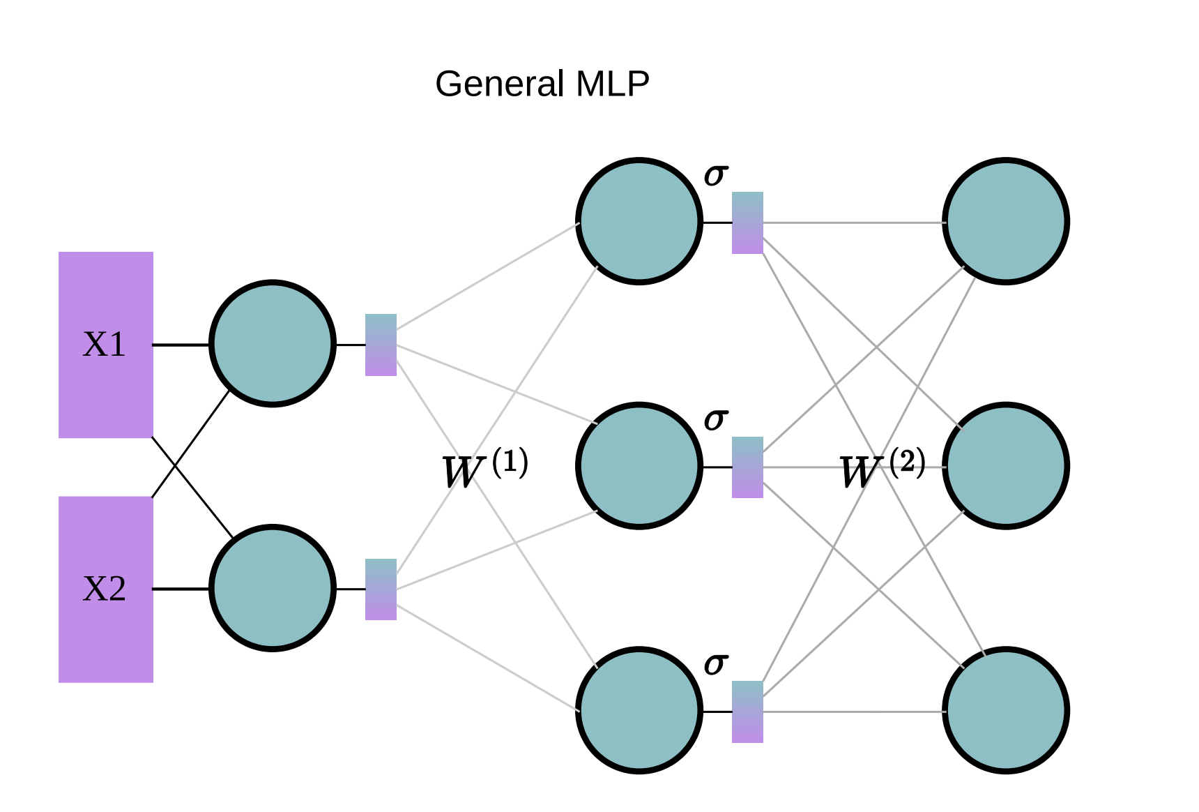
General MLP
A general MLP operates as shown in the following diagram:

The computation can be described as:
\[\text{MLP}(x) = \sigma(X{W^{(1)}}^T) W^{(2)}\]Where:
- $X$: Input data
- $W^{(1)}, W^{(2)}$: Weight matrices including all neurons
- $\sigma(\cdot)$: Activation function
Elastic MLP
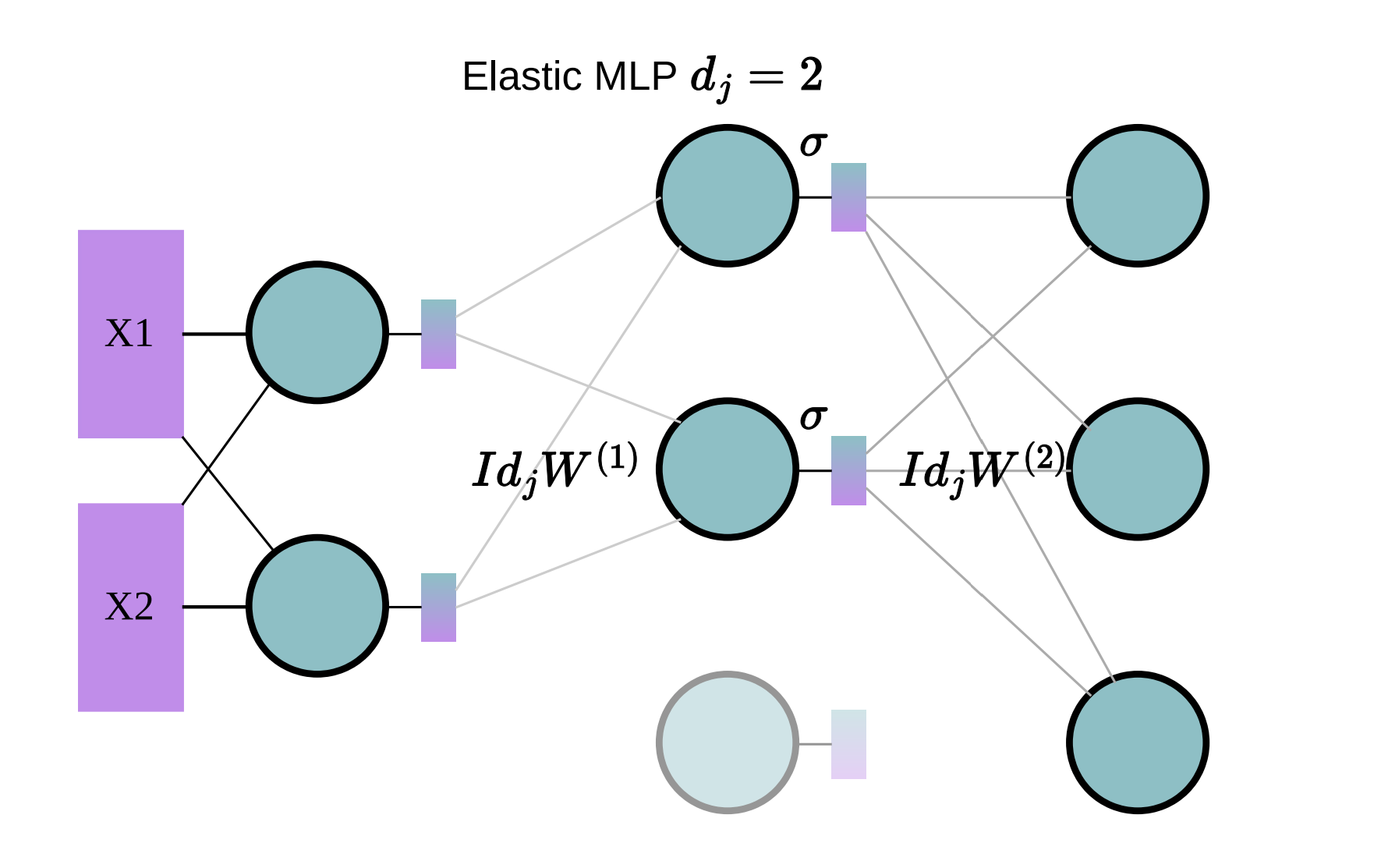
In an Elastic MLP, only a subset of neurons in the hidden layer are activated, as shown in the diagram below:

For example, the diagram illustrates the case where only 2 neurons in the hidden layer are used.
The computation for Elastic MLP is described as:
\[\text{MLP}_j(x) = \sigma(X (\text{Id}_j W^{(1)})^T) (\text{Id}_j W^{(2)})\]Where:
- $\text{Id}_j$: Activation matrix, which selectively activates the top $d_j$ neurons.
- $W^{(1)}, W^{(2)}$: Weight matrices that involve only selected neurons.
Elasitic Multi-Head Attention (MHA)
Multi-Head Attention (MHA) layers represent a significant portion of the runtime and memory usage in Large Language Models (LLMs), especially due to the Key-Value (KV) cache. Making these layers elastic can greatly enhance overall efficiency.
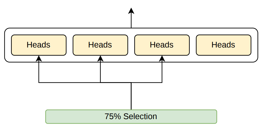
To the best of our knowledge, Flextron is the first approach that supports both elastic MLP and elastic MHA layers, offering a richer candidate operation search space. An elastic MHA candidate leverages a subset of attention heads, defined formally as follows: 
where:
- The attention head is defined as:
- $\mathbf{I}_{d_j \cdot H}$ is a diagonal matrix with the first $d_j \cdot H$ elements set to 1, and the rest set to 0,
- $d_j$ is the number of heads selected, $H$ is the size of a single head, and $L$ is the total number of heads.
The weight matrices are defined as:
\[\mathbf{W}_{Q,i}, \mathbf{W}_{K,i}, \mathbf{W}_{V,i} \in \mathbb{R}^{H \times C}, \quad \mathbf{W}_O \in \mathbb{R}^{L \cdot H \times C}.\]Different attention heads can be computed or selected dynamically using weight slicing, enabling flexible and efficient computation.
FLEXTRON Framework
Flextron introduced two concepts. Contunined-Training Process and sub-network Selection.
Elastic Network Continued-Training
Elastic continued-training optimizes LLMs by ranking and selectively training neurons and attention heads based on their importance. Here’s the process:
1. Importance Ranking
MHA Layers:
\[F_{\text{head}}(i) = \sum_{\mathbf{X}} \| \text{Attn}(\mathbf{X} \cdot \mathbf{W}_{Q,i}, \mathbf{X} \cdot \mathbf{W}_{K,i}, \mathbf{X} \cdot \mathbf{W}_{V,i}) \|_1\]MLP Layers:
\[F_{\text{neuron}}(i) = \sum_{\mathbf{X}} \| \mathbf{X} \cdot (\mathbf{W}^{(1)}_{r})^\top \|_1\]2. Elastic Layer Construction
Neurons and heads are sorted by importance. Sub-networks are created by indexing the top-ranked components, preserving critical knowledge.
3. Simultaneous Training
Candidate networks $ \mathcal{M}_j $ are trained using a combined loss:
\[\mathcal{L}_{\text{joint}} = \sum_{j=0}^{k-1} \mathcal{L}(\mathcal{M}_j(\mathbf{x}), \mathbf{y})\]Random sampling reduces the number of configurations for training, ensuring efficiency.
This approach balances scalability, efficiency, and performance by dynamically adapting LLM layers based on importance.
Automatic Network Selection
1. Problem Formulation
The objective is to minimize the cross-entropy loss while satisfying constraints:
\(\min_{\mathbf{S}_t} \sum_t \mathcal{L}_{\text{CE}}(\mathcal{M}_{s_t}), \quad \text{s.t. } \text{Latency}(\mathcal{M}_{s_t}) \leq T_t\) Here:
- $\mathcal{M}_{s_t}$ is the selected network topology for constraint $T_t$.
- \[\mathcal{G}(\mathcal{M}, \mathbf{S}_{T_t}) \text{is the function selecting} \mathcal{M}_{s_t}\]
- $\mathcal{L}_{\text{CE}}$ is the cross-entropy loss.
The optimization problem is converted using a Lagrange multiplier to:
\[\mathcal{L} = \sum_t \mathcal{L}_{\text{CE}}(\mathcal{M}_{s_t}) + \lambda \cdot \mathcal{T}_T(\mathcal{M}_{s_t})\]2. Latency Loss
Latency loss penalizes exceeding constraints:
\[\mathcal{T}_T(\mathcal{M}_{s_t}) = \sum_t \max(\text{Latency}(\mathcal{M}_{s_t}) - T_t, 0)\]3. Static Model Selection
Static routers select the number of channels/heads per layer based on latency $T$:
\[s_i = \arg\max (\mathcal{R}_i(T))\]Where $\mathcal{R}_i(T)$ is a small MLP embedding latency $T$ into logits for expert selection.
To stabilize training, a Surrogate Model (SM) predicts the LLM’s performance based on router outputs. The SM is defined as:
\[r = \text{Concat}(\mathcal{R}_0(T), \mathcal{R}_1(T), \dots, \mathcal{R}_{N-1}(T))\] \[\mathcal{S}(r) = \sigma(r \mathbf{W}_\mathcal{S}^1) \mathbf{W}_\mathcal{S}^2\]Here:
- $\mathbf{W}_\mathcal{S}^1 \in \mathbb{R}^{P \times K \cdot N}$
- $\mathbf{W}_\mathcal{S}^2 \in \mathbb{R}^{P \times 1}$
are the surrogate model weights. - $P$ is the hidden dimension.
4. Adaptive Model Selection
Dynamic routers adjust sub-networks based on both latency $T$ and hidden states $h_i$:
\[s_i = \arg\max (\mathcal{R}_i(T, h_i))\] \[\mathcal{R}_i(T, h_i) = \sigma(T \mathbf{W} + h_i \mathbf{W}_H^\top) \mathbf{W}_\mathcal{R}\]Here:
- $T$ is projected using matrix $\mathbf{W}$.
- Hidden states $h_i$ are projected into an embedding space via $\mathbf{W}_H$.
The surrogate model is extended to incorporate final hidden states $h_N$, combining latency and hidden state embeddings for token-wise routing.

The figure illustrates the process of training routers using a Surrogate Model (SM). The SM approximates the LLM’s language loss to efficiently update routers, and it is discarded after training, followed by joint fine-tuning of the LLM and routers.
