
Matryoshka Quantization
Published in , 2025
In the era of massive language models and vision transformers, model efficiency has become just as important as accuracy. Whether you’re deploying on mobile, edge devices, or scaling inference infrastructure, quantization is a crucial technique for compressing models while maintaining performance.
However, most existing quantization methods only target a single bit-width per model. If you train an INT8 model, switching to INT4 or INT2 typically requires retraining from scratch.
Google DeepMind proposes a novel solution to this inefficiency: Matryoshka Quantization (MatQuant) – a quantization technique that allows multiple bit-widths to coexist within a single model, much like Russian nesting dolls (Matryoshkas).
Background: Matryoshka Representation Learning (MRL)
The foundation of MatQuant is based on Matryoshka Representation Learning (MRL), which allows a single embedding vector to represent multiple sub-representations of different sizes. 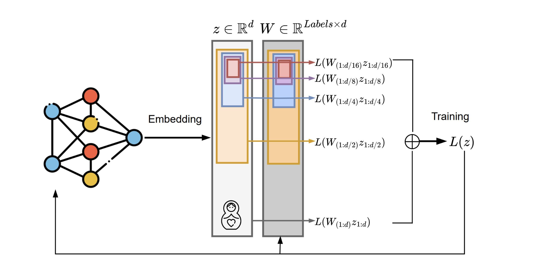 Objective Function
Each sub-representation corresponds to a slice of the full embedding (e.g., first 128, 256, or 512 dimensions), and is trained independently using its own classification head:
\[\min_{\{w^{(m)}\}{m \in \mathcal{M}},\; \theta_F} \frac{1}{N} \sum{i \in [N]} \sum_{m \in \mathcal{M}} c_m \cdot \mathcal{L} \left( w^{(m)} \cdot F(x_i; \theta_F)_{1:m},\; y_i \right)\]Where:
$F(x_i; \theta_F)_{1:m}$: the first m dimensions of the embedding for input x_i
$w^{(m)}$: classifier for the m-dim sub-embedding
$c_m$: importance weight for each embedding size
The total loss is a weighted sum of these individual classification losses, enabling the model to support multiple representation sizes at once.
Nested Embedding: Coarse-to-Fine Information
Before training, information in the embedding is uniformly distributed. After MRL, however, important information becomes concentrated in the earlier dimensions, forming a coarse-to-fine hierarchy. 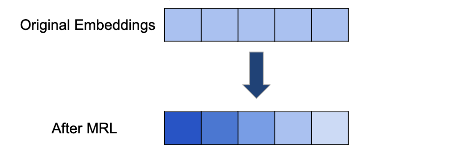
This allows for adaptive inference:
In low-resource settings, only the first few dimensions can be used.
For high-performance scenarios, the full embedding can be utilized.
Quantization Base: QAT and OmniQuant
Matryoshka Quantization builds upon standard quantization techniques, primarily:
QAT (Quantization-Aware Training)
QAT simulates quantization during training so the model can learn to be robust to quantized inference.
The most common technique is MinMax Quantization:
\[Q_{\text{MM}}(w, c) = \operatorname{clamp}\left(\left\lfloor \frac{w}{\alpha} + z \right\rceil,\; 0,\; 2^c - 1\right)\] \[\alpha = \frac{\max(w) - \min(w)}{2^c - 1},\quad z = -\frac{\min(w)}{\alpha}\]OmniQuant
OmniQuant takes a different approach: instead of updating weights, it learns auxiliary parameters that minimize the difference between full-precision and quantized outputs.
Objective:
\[\min_{\gamma, \beta, \delta, s} \left\| F_l(W_F^l, X_l) - F_l(Q_{\text{Omni}}(W_F^l), X_l) \right\|_2^2\]- Weight Quantization:
- Activation:
Here, $\gamma$, $\beta$, $\delta$, $s$ are all learnable parameters that allow adaptive clipping and scaling.
Matryoshka Quantization (MatQuant)
The core idea of MatQuant is bit-slicing – extracting the top bits from a quantized tensor to simulate lower-bit models from higher-bit weights.
Bit-Slicing Formula: 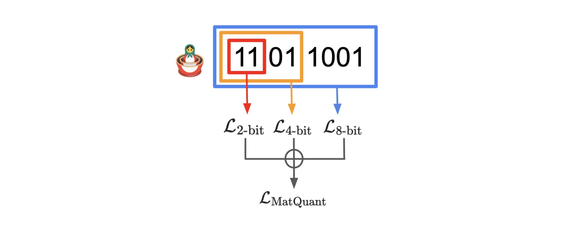
Where:
$q^c$: c-bit quantized weights
$r$: number of most significant bits (MSBs) to keep
Bit-slicing allows the same model to function as INT2, INT4, INT8 simply by adjusting how many bits are read from each weight.
Multi-Bit Training
MatQuant optimizes models across multiple bit-widths simultaneously using QAT or OmniQuant.
QAT + MatQuant:
\[\mathcal{L}_{\text{total}} = \sum_r \lambda_r \cdot \mathcal{L}{\text{CE}}\left(S(Q(\theta, c), r),\; y\right)\]OmniQuant + MatQuant:
\[\mathcal{L}{\text{total}} = \sum_r \lambda_r \cdot \left\| S(Q{\text{Omni}}(W^l_F, c), r) - F_l(W^l_F, X_i^l) \right\|^2\]Each bit-width contributes a separate loss, and all are jointly optimized with weight $\lambda_r$.
Quantized Results
MSB-focused Distribution
Unlike conventional quantization, MatQuant shifts weight distribution so that more information resides in the most significant bits (MSBs). 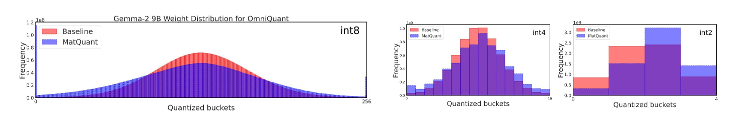
In comparison to the OmniQuant baseline:
MatQuant’s INT8, INT4, INT2 distributions show higher concentration of 1s in the upper bits.
This structure mirrors MRL, where earlier embedding dimensions carried the most meaningful information.
Interpolative Behavior
MatQuant is trained only on INT8, INT4, and INT2. Still, it generalizes naturally to unseen bit-widths like INT6 and INT3.
This is due to:
The nested bit structure
The consistent information density in the upper bits